Case Study: Convection at High Earth Altitudes

Introduction

The Columbia Scientific Balloon Facility (CSBF) is a NASA facility responsible for providing launch, tracking and control, airspace coordination, telemetry and command systems, and recovery services for unmanned high-altitude balloons. To simulate the conditions experienced by the equipment during flights, computer simulations are run using C&R Technologies’ Thermal Desktop. The focus of this semester’s research is to determine the impact of convective heat transfer during missions and if it is necessary to include in future models.

Methodology

The piece of equipment under observation is the Support Information Package (SIP) Shield. Composed of insulation foam, the SIP Shield is necessary to protect a variety of electrical components from the extreme temperatures present at altitudes of 120 kft. Figure 1 graphically displays how the air temperature varies throughout the stratosphere and troposphere.

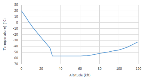
Figure 1. Atmospheric air temperature versus altitude graph [1]

To compute the convection coefficients present at varying altitudes, first the thermophysical properties of air were documented from the U.S. Standard Atmosphere 1976 manual. Using the programming language, FORTRAN, these values were coded as functions of altitude so that would update as the balloon ascends.

Figure 2. Code example: Air density as function of altitude

Using Thermal Desktop, the SIP Shield was modeled as a 6-sided box measuring 20” x 30” x 50” while the thickness of each face is approximately 1/12”. While in flight the shield is surrounded by various other members of the payload, most prominently the gondola and truss. Their respective geometry has been simplified to two rectangular plates while the atmospheric air was represented as a boundary node.

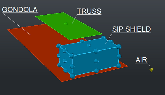
Figure 3. Thermal Desktop model

The geometry for the SIP Shield is a combination of vertical and horizontal plates, where the top and bottom were defined as horizontal and the remaining vertical. Computations for these convective coefficients can be found in the Appendix. To add these characteristics to model, each of the outer surfaces were coupled to the boundary air node and assigned the proper convection variable.

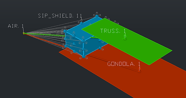
Figure 4. Convection couplings

Radiation was computed by coupling sections of the geometry into radiation analysis groups. Only objects in these group will be consider during the radiation calculations. For this model, the group was named, “Exterior.” As the name suggests only the exterior faces of the SIP Shield were included along the top and bottom faces of the gondola and truss. Though not visible in the model, a pseudo node representing space is also incorporated into the programs computations. The SIP Shield is typically coated in white paint, aluminum tape, or a combination of the two. The truss and gondola for this study were covered with white paint.

The locations under review are Wanaka, New Zealand and the McMurdo Station in Antarctica which are popular launch sites for the CSBF. For each location, the balloon will undergo a geosynchronous orbit at its respective latitude. This experiment is divided up into 3 cases; ground, ascent, and float. The ground case is a steady state problem where the SIP Shield is resting on the launch pad. The ascent case involves the balloon rising at a constant rate from the ground to 120 kft over the course of 3 hours. Lastly, the float case is a 24 hours transient case at a constant altitude of 120 kft.

Figure 5. Wanaka, New Zealand geosynchronous orbit

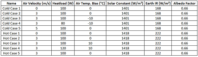
A series of experiments were ran to assist in the evaluation of convection. Tables 1 and 2 document the varying parameters of each case. The air velocity indicates the presence of forced convection and is used in the computing the convective couplings. Next, the heat load is the wattage generated by the interior components of the SIP, thus heating the shield. Air Temp Bias is a variable used to alter the entire air temperature profile seen in Figure 1. For example, a value of 10°C would shift each of the y-values upward 10°C. The following three parameters are used to calculate radiative effects based on the location of the flight.

Table 1. Wanaka, New Zealand case descriptions

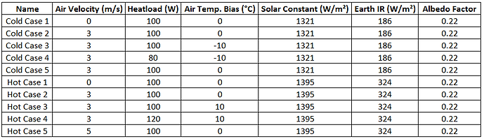
Table 2. McMurdo, Antarctica case descriptions

Results

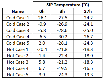
Figures 6 and 7 present the SIP Shield temperatures occurring from the end of the steady state ground case to end of the float case, totaling to 27 hours. In addition, Tables 3 and 4 show the abridged temperature results measured at the end of the ground, ascent, and float runs.

Figure 6. Wanaka, New Zealand flight temperature distribution

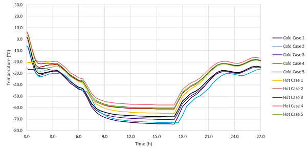
Figure 7. McMurdo, Antarctica flight temperature distribution

Table 3. Wanaka, New Zealand abbreviated data

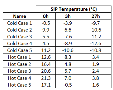
Table 4. McMurdo, Antarctica abbreviated data

Conclusions

At ground level, convection is quite dominate, however, as the SIP Shield rises in altitude its effects greatly diminish. Figure 8 demonstrates this claim by displaying the difference between cold cases 1 and 2 and hot cases 1 and 2 for each location. Since the first two cases contain identical conditions aside from the presence of convection, the impact of this form of heat transfer can be seen by examining the deviation between them.

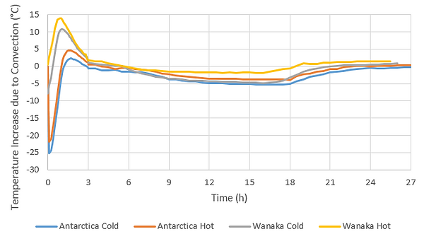
Figure 8. Temperature difference between cases 1 and 2

During the ascent portion, the absolute temperature difference appears to be at its largest. For the Wanaka cases, the convection causes the most increase at about 1h. Here, the SIP Shield is approximately at the transition point (about 33 kft) between the troposphere and stratosphere, where the air temperature abruptly sinks. Once the SIP reaches float altitude, the difference appears to settle into a pattern oscillating between 0°C and up to 5°C. In conclusion, these case studies appear to reinforce the notion that convective heat transfer is negligible at high altitudes.

References

[1] Dewitt, D., 2011, Fundamentals of Heat and Mass Transfer 7e, John Wiley & Sons, Hoboken, New Jersey.

[2] United States Committee on Extension to the Standard Atmosphere, 1976, “U.S. Standard Atmosphere, 1976,” National Oceanic and Atmospheric Administration.

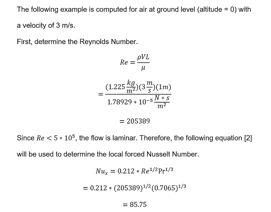
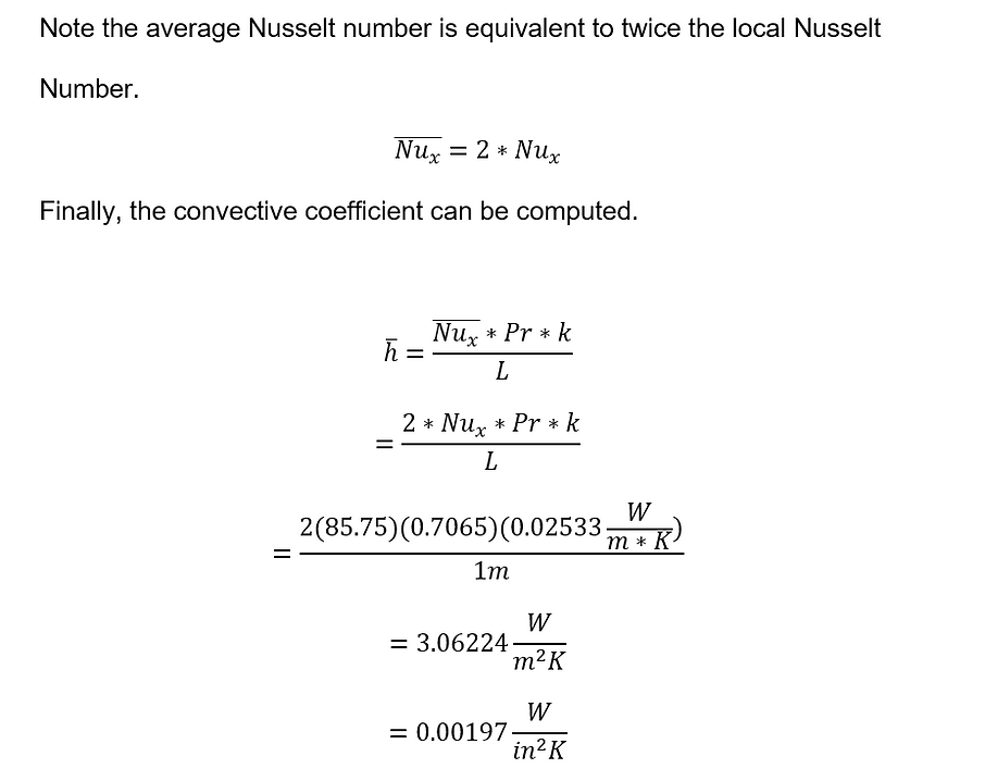
Appendix: Convection Calculations

Zachary Schaetz